Both financial and managerial accounting classify, record, and report an organization’s financial activity, but they exist to serve completely different audiences. Financial accounting is aimed at external users – investors, creditors, and regulators – and is therefore standardized by bodies such as the Financial Accounting Standards Board and the Securities and Exchange Commission, so that outsiders can compare one company’s reports against another’s using a common set of rules. Managerial accounting, by contrast, is built for internal decision makers – the managers who plan, control, and evaluate day-to-day operations – and because no outside regulator ever sees these reports, they are customized freely to whatever format is most useful for a specific decision, whether that means a cost report broken down by product line, a monthly departmental budget, or a one-off analysis of whether to accept a special order.
Product Costs vs. Period Costs
Every cost an organization incurs is classified as either a product cost or a period cost, and the distinction matters because product costs are capitalized into inventory on the balance sheet until the related goods are sold, while period costs are expensed immediately in the period they are incurred. For a merchandising business – one that buys finished goods and resells them, such as a retail store – product cost is simply what the business paid to acquire the inventory, while period costs cover everything else needed to run the business: rent, utilities, wages, and advertising. For a manufacturer, product costs are broader because the business is creating the inventory rather than buying it finished, and they split into three categories: direct materials (raw materials that can be traced economically to a specific unit, such as the fabric in a jacket), direct labor (wages of workers who physically build the product), and manufacturing overhead (every other indirect production cost that cannot be traced to a specific unit, such as factory rent, the supervisor’s salary, or glue and other minor supplies).
Cost Behavior: Fixed, Variable, and Mixed Costs
Cost behavior describes how a cost responds to changes in the level of production or sales activity, and every cost falls into one of three behavior patterns. A variable cost stays the same on a per-unit basis, but its total rises and falls with the chosen activity driver – the measure that causes the cost, such as units produced or machine hours used. A fixed cost is the mirror image: its total stays the same regardless of activity, but the amount allocated to each unit shrinks as volume rises. A mixed cost contains both a fixed and a variable piece at once. Consider a small bakery that rents a kiosk for $2,800 a month and buys flour and packaging that cost $0.60 per loaf sold. The kiosk rent is fixed – it is $2,800 whether the bakery sells 200 loaves or 2,000 – but the per-loaf rent allocation drops from $14.00 at 200 loaves to $1.40 at 2,000 loaves. The flour and packaging cost is variable – always $0.60 per loaf – so total ingredient cost is $120 at 200 loaves and $1,200 at 2,000 loaves. If the bakery’s monthly electricity bill includes a flat base charge plus a per-kilowatt-hour usage charge that rises with how much baking the ovens do, that utility bill is a mixed cost.
The Relevant Range of Production
Fixed and variable cost behavior only holds true within a specific band of activity called the relevant range – the span between a minimum and maximum production level over which the organization’s existing capacity and cost structure remain valid. Inside that range, a manager can reliably predict costs using the fixed-plus-variable logic described above. Outside it, the assumptions break down: pushing production past the top of the relevant range might require leasing a second kiosk or buying a second oven, which would step the fixed cost up to a new, higher level rather than letting it stay constant. A manager estimating costs for a proposed expansion always needs to check first whether the new volume still falls inside the range where current cost relationships apply.
The High-Low Method for Predicting Mixed Costs
When a cost is mixed and a manager needs to split it into its fixed and variable components, the high-low method offers a quick four-step estimate using only the highest and lowest activity observations in a set of historical data. Suppose a print shop’s mixed equipment maintenance cost was $1,340 in its highest-activity month, when it ran 2,150 print jobs, and $980 in its lowest-activity month, when it ran 1,400 print jobs. Step one finds the difference: 750 jobs and $360 in cost. Step two divides the cost difference by the activity difference to estimate variable cost per job: $360 divided by 750 equals $0.48 per job. Step three applies that variable rate back to either observation to isolate the fixed component – using the high month, 2,150 jobs times $0.48 equals $1,032 in variable cost, and subtracting that from the $1,340 total leaves $308 in fixed cost per month (the low month produces the same $308 figure, which confirms the calculation). Step four assembles the cost formula in the standard Y = a + bx form, where Y is total cost, a is the fixed component, b is the variable rate, and x is the activity level: Y = $308 + $0.48x. That formula can then estimate maintenance cost at any volume within the shop’s relevant range.
Traditional vs. Contribution Margin Income Statements
An income statement reports an organization’s revenue less its expenses for a period, and net operating income comes out the same regardless of which format is used – the two formats differ only in how they organize the expense side. A traditional income statement organizes costs by function, separating product costs (cost of goods sold) from period costs (selling and administrative expenses), and it is the format used for external financial reporting because it aligns with the product-cost and period-cost distinction required under generally accepted accounting principles. A contribution margin income statement instead organizes costs by behavior, separating variable costs from fixed costs, and subtracting total variable costs from sales revenue to arrive at contribution margin before fixed costs are deducted. Because it isolates variable costs, the contribution margin format is the one managers use internally for cost volume profit analysis, break-even calculations, and short-term decisions such as whether to accept a one-time special order, none of which the traditional format is built to support directly.
Quick Revision Summary
Financial accounting serves external users under standardized rules; managerial accounting serves internal decision makers with customized, unregulated reports. Product costs attach to inventory until sale; period costs expense immediately. A manufacturer’s product costs split into direct materials, direct labor, and manufacturing overhead. Variable costs are constant per unit but change in total with activity; fixed costs are constant in total but change per unit; mixed costs combine both, and the high-low method isolates their fixed and variable components using only the highest and lowest activity observations. Cost predictions using fixed and variable behavior only hold within the relevant range of production. A traditional income statement classifies costs as product or period for external reporting, while a contribution margin income statement classifies costs as variable or fixed for internal planning and decision making, and both formats always report the same bottom-line net operating income.
Payroll is the process of administering employees’ pay, and it stretches back further than most business functions – clay tablets from roughly 3000 BCE already recorded worker pay in rations, which is a reminder that keeping accurate pay records is one of the oldest administrative tasks in human commerce. Today payroll has grown into a specialized, software-driven function precisely because the legal requirements around it have grown more complex: a Canadian payroll professional has to track federal rules that apply everywhere in the country alongside provincial or territorial rules that differ from one jurisdiction to the next, and both layers change periodically as legislation is updated. Getting payroll right matters for two distinct audiences. Employers rely on accurate payroll to remain compliant with the Canada Revenue Agency and to offer competitive, correctly calculated compensation, while employees rely on payroll to understand exactly how their gross pay becomes net pay and to trust that the withholdings taken from every cheque are being remitted on their behalf.
What the Payroll Function Actually Does
Payroll is often assumed to be a simple matter of multiplying hours by a wage rate, but the function carries a long list of responsibilities that touch nearly every stage of the employment relationship. Payroll professionals confirm with management how much and how often an employee should be paid, verify timesheets or hours worked, calculate gross pay, and then adjust that figure for lump sum payments, accrued severance, vacation and personal days, sick leave, and leaves of absence. From there, payroll determines which withholdings the law and any applicable agreements require, deducts insurance or benefit premiums where relevant, and arrives at each employee’s net pay. The function also extends beyond the individual paycheque: payroll calculates and remits statutory holiday pay, produces a Record of Employment whenever an employee’s earnings are interrupted for more than thirteen weeks, determines and remits the employer’s own payroll expenses to the CRA, maintains complete pay records for every employee, and verifies each employee’s T4 information before year-end slips are issued. Because legislation changes periodically, payroll must also update its own processes and policies every year to stay compliant.
Setting Up a Payroll Account with the CRA
Any individual or organization that will pay one or more employees must register a payroll account with the Canada Revenue Agency before the first remittance of deductions or employer expenses comes due. That payroll account sits underneath the organization’s business number, a unique nine-digit identifier used for every CRA program account the organization holds, so the payroll account functions as a sub-account of the BN rather than a separate identity. A business number can be obtained by registering online through the CRA’s Business Registration Online service, by mailing in the RC1 form, or automatically as part of incorporating a business in most provinces outside Quebec and Newfoundland. An organization that operates in more than one province, or that runs more than one distinct business activity, may register multiple payroll accounts under the same BN, but the underlying rule stays simple: one business number per legal entity, with as many payroll sub-accounts as its structure requires. Employers must also set up accounts with other payees where relevant, such as provincial workers’ compensation boards and employer health tax programs.
Manual Payroll, Software, or Outsourcing
Canadian employers can legally run payroll manually, but the CRA’s electronic filing rules push most organizations toward software once they cross a small size threshold: employers filing six or more information returns (T4 slips) in a year are required to file electronically, and the penalty for failing to do so scales with the number of returns involved, running from a modest fine for a handful of missed slips up to several thousand dollars for organizations filing thousands of returns. Employers with up to roughly 100 employees can often satisfy this requirement using the CRA’s web forms rather than purchasing dedicated software, but beyond that volume, most organizations need software capable of encoding return data for submission through internet file transfer. Beyond the electronic filing threshold, the decision to use payroll software, and which software to choose, depends on organizational size, whether payroll staff work remotely, how complex the organization’s pay calculations and benefits are, how many jurisdictions the organization operates in, and how much automation and integration with other HR functions the organization wants. Smaller, single-jurisdiction employers can often manage with simpler tools, while larger or multi-jurisdictional employers typically need software built to handle jurisdiction-specific tax rules and higher data volumes. Outsourcing payroll entirely is common among smaller organizations with limited in-house capacity, rapidly growing organizations whose payroll needs are outpacing their internal systems, and organizations with complex, multi-jurisdictional payroll.
Onboarding a New Employee Into Payroll
Setting up an individual employee in the payroll system requires collecting and validating several pieces of information before that employee’s first pay run. A Social Insurance Number must be obtained from every new employee, who has three days from their start date to provide it (or three days from receiving a newly issued SIN if they did not already have one); employers are not permitted to request a SIN before extending an offer of employment. Temporary residents carry SINs beginning with the digit nine, and those numbers carry an expiry date that payroll must track, since an expired or incorrectly recorded SIN can disrupt an employee’s access to government benefits down the line. Every new employee must also complete a TD1 Personal Tax Credits Return, both federal and provincial, which determines how much of their income qualifies for the basic personal deduction and any additional credits tied to dependents, tuition, or disability status; an employee must update their TD1 within seven days of any personal change that affects it, and an employee working more than one job at once must still file a TD1 with each employer but cannot claim the same credit amounts twice.
Recording the Correct Province of Employment
Because provincial and territorial tax rules differ, payroll must record the correct province or territory of employment for every worker, since this determines which T4 is issued and which provincial withholding tables apply. The governing rule depends on the nature of the work: an employee who physically reports to a single workplace is recorded in the province where that workplace is located; an employee working remotely is generally recorded in the province where the employer’s payroll records are kept, which is often but not always where the employee happens to be sitting; and an employee who genuinely works in more than one province or territory during the year must have a separate T4 issued for each region in which they worked. Payroll professionals are not responsible for setting an employee’s rate of pay – that is negotiated through an employment contract for non-unionized staff or a collective agreement for unionized staff – but they are responsible for administering payroll strictly according to whichever agreement governs that employee, and for flagging any apparent error, such as a rate below the applicable statutory minimum wage, to the appropriate manager rather than silently processing it.
Quick Revision Summary
Payroll is the administration of employee pay, including deductions, withholdings, and remittances, and it exists to keep employers compliant with the CRA while giving employees a clear, correct record of how gross pay becomes net pay. Every employer with at least one employee must register a payroll account, which sits as a sub-account under the organization’s business number, before its first remittance is due. Employers filing six or more T4 slips must file electronically, with penalties for non-compliance rising with the number of returns involved; this threshold, combined with organizational size, jurisdictional spread, and payroll complexity, generally drives the choice between manual payroll, software, and outsourcing. Onboarding a new employee requires a validated SIN within three days of the start date and a completed TD1 form determining personal tax credits, and every employee’s province of employment must be recorded accurately – by workplace location for in-person staff, by payroll’s location for remote staff, and separately for each province where an employee genuinely works in more than one.
Why Managerial Accounting Ends With Present Value Tables
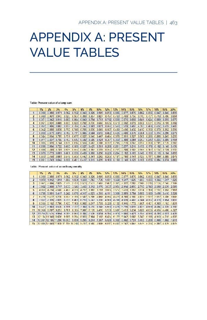
A managerial accounting course builds toward capital budgeting, and capital budgeting decisions – should the company buy the new machine, open the new location, replace the old delivery fleet – all hinge on comparing cash that arrives at different points in time. A dollar received five years from now is worth less than a dollar in hand today, because today’s dollar can be invested and grow. Present value tables exist to make that comparison mechanical rather than requiring a fresh formula calculation every time: instead of computing (1 + i)^-n by hand for every discount rate and time horizon a course might ask about, a student looks up the intersection of a discount rate column and a number-of-periods row and reads off a present value factor, then multiplies that factor by the future cash amount.
Reading a Present Value of $1 Table
The first table used in capital budgeting problems shows the present value of a single lump-sum amount of $1 received at the end of a given number of periods, discounted at a given interest rate. To use it, a student locates the row for the number of periods until the cash is received and the column for the discount rate (the company’s required rate of return, sometimes called the hurdle rate), and the factor at that intersection is multiplied by the actual future cash amount to find its value in today’s dollars. For example, if a table shows a factor of 0.7130 for eight periods at 7 percent, a future receipt of $10,000 in eight years would have a present value of $7,130 today at that discount rate. This single-sum table is the one used for calculating the present value of a machine’s salvage value at the end of its useful life, or any other one-time cash flow that occurs at a specific future date rather than repeating every period.
Reading a Present Value of an Annuity Table
The second table covers an annuity – a series of equal cash flows occurring at the end of each period for a set number of periods, such as the annual net cash inflow a new machine is projected to generate every year of its useful life. Rather than looking up a separate single-sum factor for each year’s cash flow and adding eight numbers together, the annuity table collapses that entire stream into one factor for a given number of periods and discount rate. Multiplying that single factor by one period’s cash flow amount (assuming the amount is the same every period) gives the present value of the whole stream at once. This is the table used in net present value calculations for a piece of equipment expected to generate a steady annual cash inflow, and it is also the table underlying loan amortization and annuity-due problems in a corporate finance course.
How the Glossary Ties the Course Together
The glossary that accompanies a managerial accounting text is best read as a map of the course’s four major units rather than a list to memorize term by term. The first unit, cost behavior, distinguishes a fixed cost – one whose total dollar amount does not change as production volume rises or falls, such as monthly factory rent – from a variable cost, whose total rises and falls with volume even though the per-unit amount stays constant, such as the cost of raw material per unit produced. A mixed cost blends both patterns, which is why the high-low method exists: it isolates the variable and fixed components of a mixed cost by comparing the highest and lowest activity levels observed and treating the difference in total cost as attributable entirely to the change in volume.
Costing Systems and Manufacturing Accounts
The second unit covers how a manufacturer assigns cost to what it produces. Job-order costing tracks direct material, direct labor, and manufacturing overhead separately for each distinct job or batch, recording the totals on a job cost sheet, and it suits businesses that produce customized or low-volume output such as custom furniture or construction projects. Manufacturing overhead itself is every production cost that cannot be traced directly to a specific unit – the factory supervisor’s salary, factory utilities, machine depreciation – and because these costs cannot be traced directly, businesses apply them to jobs using a predetermined overhead rate calculated in advance by dividing estimated total overhead by an estimated allocation base such as direct labor hours or machine hours. As production happens, cost flows through three inventory accounts in sequence: Raw Materials, then Work in Process as material, labor, and applied overhead accumulate on unfinished units, and finally Finished Goods once a job is complete and ready for sale.
Budgeting and Variance Terminology
The third unit shifts from historical costing to forward planning. A master budget is the umbrella term for the full set of interlocking budgets – sales, production, materials purchases, manufacturing overhead, and selling and administrative expenses – that together forecast an organization’s financial position for a future period. A planning budget is prepared before the period begins, using the sales volume management expects to achieve, while a flexible budget takes the same cost formulas but reforecasts them using the volume the organization actually achieved, which makes the flexible budget a fairer benchmark for judging cost control than the original planning budget. Comparing the planning budget to the flexible budget isolates an activity variance, caused purely by selling a different quantity than planned, while comparing the flexible budget to actual results isolates a revenue or spending variance, caused by prices or efficiency that differed from what was budgeted for the volume actually achieved.
Performance Evaluation by Segment
The fourth unit applies these same cost-behavior ideas to evaluating parts of an organization rather than the whole. Segmented income reporting traces revenue and variable costs to the specific division, store, region, or product line that generated them, and fixed costs are split into traceable fixed costs (attributable to one segment, and which would disappear if that segment were eliminated) and common fixed costs (shared across segments, such as the CEO’s salary, which would not disappear even if one segment were dropped). Subtracting a segment’s traceable fixed costs from its own contribution margin yields its segment margin, which is the figure managers use to judge whether a segment is pulling its weight, since it strips out costs the segment’s own operations do not actually control.
Quick Revision Summary
A present value of $1 table converts a single future lump sum into today’s dollars by multiplying the future amount by the table factor found at the intersection of the discount rate and number of periods; a present value of an annuity table does the same for a level, repeating cash flow stream in one step. Fixed costs stay constant in total as volume changes, variable costs stay constant per unit, and mixed costs contain both elements. Job-order costing assigns direct material, direct labor, and applied manufacturing overhead to each job as it moves through Raw Materials, Work in Process, and Finished Goods. A flexible budget restates the planning budget at actual volume, separating activity variances (caused by volume) from revenue and spending variances (caused by price and efficiency). Segment margin equals a segment’s contribution margin minus its own traceable fixed costs, deliberately excluding the common fixed costs the segment does not control.
Every amount withheld from an employee’s gross pay falls into one of three groups, and a payroll clerk needs to know which group a deduction belongs to before deciding how it is calculated, remitted, and reported. The first group is statutory (source) deductions, which every employer in Canada is legally required to withhold regardless of what the employee wants: Canada Pension Plan contributions, Employment Insurance premiums, and federal and provincial income tax. The second group is other mandatory deductions, which are still compulsory but arise from a specific legal order or circumstance rather than applying automatically to every paycheque – a Requirement to Pay issued by the Canada Revenue Agency, a court-ordered wage garnishment, a family support order, or union dues owed under a collective agreement. The third group is non-mandatory (voluntary) deductions, which only come off pay because the employee has agreed to them in writing – health and dental premiums, life insurance, contributions to a registered pension plan above the mandatory minimum, or a payment redirected to a credit union. Getting this classification right matters because the legal remedy for an employer who withholds too little differs sharply between the three: shortfalls in statutory deductions expose the employer to CRA penalties and interest, while an unauthorized voluntary deduction can expose the employer to an employment standards complaint.
Canada Pension Plan Contributions
CPP is designed so that contributions are shared equally between employee and employer, and the calculation starts with a basic exemption of $3,500 per year, which is prorated across pay periods so that a small slice of each paycheque is contribution-free before CPP is applied to the remainder. Above the exemption, contributions apply up to the Year’s Maximum Pensionable Earnings, which was $71,300 for 2025, at a combined base-plus-enhanced rate of 5.95 percent on the employee side for 2024 (employers match this dollar for dollar). Since 2024, a second tier – CPP2 – applies an additional 4 percent employee contribution on earnings between the YMPE and a second, higher ceiling, which was $81,200 for 2025. This second tier exists because the CPP enhancement was phased in specifically to lift the income replacement rate for higher earners, and it only touches the portion of an employee’s annual earnings that falls in that upper band. Once an employee’s cumulative contributions for the year reach the annual maximum, no further CPP should be withheld from that employer for the remainder of the year, which is why payroll software tracks year-to-date CPP contributions per employee rather than simply applying the rate to every cheque in isolation.
Calculating CPP – A Worked Example
Suppose an employee named Priya is paid bi-weekly (26 pay periods a year) with gross earnings of $2,400 for the period. The bi-weekly basic exemption is $3,500 divided by 26, which comes to $134.62. Subtracting that from gross pay leaves $2,265.38 of pensionable earnings for the period. Applying the 5.95 percent base-plus-enhanced rate gives an employee CPP contribution of $134.79 for that pay period, and the employer contributes the identical amount. If Priya’s year-to-date pensionable earnings later cross the $71,300 YMPE threshold, any additional earnings up to $81,200 would instead attract the separate 4 percent CPP2 rate rather than the regular 5.95 percent rate, and once cumulative CPP2 contributions reach their own annual maximum, withholding would stop for that tier as well. This two-tier structure means a payroll clerk preparing a manual calculation late in the calendar year for a highly paid employee needs to check both YTD figures – regular CPP and CPP2 – before applying a rate, rather than assuming the same 5.95 percent applies to every dollar all year.
Employment Insurance Premiums
EI premiums are calculated only on the employee side up to an annual maximum insurable earnings ceiling, with the employer contributing 1.4 times whatever the employee pays – a ratio set in legislation to reflect that employers are the ones who lay off staff and therefore fund a larger share of the program. For 2024 the employee premium rate was 1.66 percent of insurable earnings, producing a maximum annual employee premium of $1,049.12, which rose to $1,077.48 for 2025 as the insurable earnings ceiling increased. Unlike CPP, EI has no basic exemption – the rate applies from the first dollar of insurable earnings. Using the same bi-weekly employee, Priya, with $2,400 of insurable earnings in a pay period, the EI premium is $2,400 multiplied by 1.66 percent, which comes to $39.84 for the period, and the employer’s matching share is $39.84 multiplied by 1.4, or $55.78. As with CPP, once an employee’s cumulative EI premiums for the calendar year reach the annual maximum, the employer stops withholding EI for the rest of the year, even if the employee changes jobs partway through and a new employer would otherwise start the calculation over.
Income Tax Withholding
Federal and provincial income tax withholding is the most complex of the three statutory deductions because, unlike CPP and EI, it is not a flat percentage – it depends on the employee’s total annual income, the province of employment, the personal tax credits claimed on their TD1 forms, and any additional voluntary withholding the employee has requested. In practice, few payroll professionals calculate income tax by hand; the Canada Revenue Agency’s Payroll Deductions Online Calculator (PDOC) is the standard tool, and it produces a defensible, auditable withholding figure once the employee’s gross pay, pay period frequency, province, and TD1 claim amounts are entered. Because income tax brackets are progressive, the calculator effectively annualizes the pay period’s earnings to estimate which bracket the employee falls into, then converts that back down to a per-period withholding amount, which is why doubling a bi-weekly pay period’s gross pay does not simply double the tax withheld.
Other Mandatory Deductions
Beyond the three statutory deductions, an employer may be legally compelled to withhold further amounts. A Requirement to Pay is a formal notice from the CRA directing an employer to redirect an employee’s wages toward that employee’s outstanding tax debt; ignoring it makes the employer personally liable for the unpaid amount. Where an employer provides meals or lodging as part of employment, the value of that benefit is subject to prescribed deduction caps rather than being treated as fully taxable at cost. Court-ordered wage garnishments and family support orders are administered provincially and the rules differ meaningfully by jurisdiction: in Alberta, a garnishment order must leave the employee with at least $800 of net pay exempt from seizure, while family support enforcement bodies operate on separate ceilings – Ontario’s Family Responsibility Office can direct up to 50 percent of an employee’s net income toward support arrears, and Alberta’s Maintenance Enforcement Program can direct up to 40 percent of gross income. An employer served with more than one garnishment or support order at once generally must satisfy support orders ahead of ordinary creditor garnishments, and payroll staff should never assume the caps are interchangeable across provinces.
Union Dues and Pension Plan Contributions
Where a workplace is unionized, dues are typically mandatory under what is known as the Rand Formula, a principle from Canadian labour law holding that because all employees in a bargaining unit benefit from a collective agreement, all employees – whether or not they choose to join the union – must contribute dues that fund the union’s representation of the unit. This makes union dues a mandatory deduction even for a non-member employee covered by the agreement. Registered pension plan contributions can sit in either the mandatory or voluntary category depending on plan design: where an employer’s defined benefit or defined contribution plan requires participation as a condition of employment, the minimum contribution is mandatory, while any additional voluntary contribution an employee elects to make on top of that minimum falls into the third category discussed below.
Non-Mandatory (Voluntary) Deductions
Voluntary deductions only leave an employee’s pay because the employee has given written authorization, and an employer that deducts an amount in this category without that authorization risks an employment standards complaint. Common examples include premiums for employer-sponsored health and dental benefit plans, supplemental life or disability insurance, contributions to a workplace charitable giving program, and wage assignments – a standing instruction to redirect part of pay to a third party such as a credit union. Provincial rules cap how much of an employee’s pay can be redirected this way: in Ontario, a wage assignment to a credit union is generally capped at 20 percent of wages, while British Columbia, Yukon, and Alberta apply their own variations on the permissible cap and process. Because these deductions are optional, an employee can generally revoke the authorization going forward, and the employer must stop the deduction from the next practical pay period once notified, unlike statutory or court-ordered deductions, which continue regardless of the employee’s wishes.
Quick Revision Summary
Payroll deductions split into three categories: statutory (CPP, EI, income tax – compulsory for every employee), other mandatory (RTP, garnishments, support orders, union dues – compulsory once triggered by a legal order or agreement), and non-mandatory (health plans, extra insurance, wage assignments – only with the employee’s written consent). CPP for 2025 applies at 5.95 percent above a $3,500 basic exemption up to the $71,300 YMPE, with a further 4 percent CPP2 tier up to $81,200. EI for 2024 applied at 1.66 percent from the first dollar up to a $1,049.12 annual maximum, rising to $1,077.48 for 2025, with employers matching at 1.4 times the employee premium. Income tax withholding is calculated through the CRA’s PDOC tool rather than a flat rate. Garnishment and support-order limits vary by province – Alberta preserves an $800 exemption on garnishments, Ontario’s FRO can reach 50 percent of net income, and Alberta’s MEP can reach 40 percent of gross income – so payroll staff must apply the rule of the province where the employee is paid, not a single national figure.
Cost volume profit, or CVP, analysis gives managers a structured way to answer one of the most common questions in business: how will a change in price, cost, or sales volume actually move the bottom line. Rather than guessing, CVP analysis uses the relationship between an organization’s fixed costs, variable costs, selling price, and sales volume to predict the effect of a proposed decision before it’s made, whether that decision is a price cut, a new marketing push, a switch to higher-quality materials, or simply figuring out how many units need to sell before the business turns a profit at all.
What CVP Analysis Is Used For
CVP analysis exists to answer one core question: how do changes in selling price, sales volume, variable cost per unit, total fixed costs, or the mix of products sold affect net operating income. Because these five factors interact, a decision that looks good on one dimension, cutting price to boost volume, say, can still hurt overall profit if the volume increase isn’t large enough to offset the lower margin per unit, and CVP analysis is the tool that quantifies exactly how large an increase would need to be.
This makes CVP analysis central to decisions like setting prices, evaluating a proposed increase to the advertising budget, deciding whether a cost structure with more fixed costs and lower variable costs (or vice versa) suits the business better, and figuring out the sales volume a new product needs to reach before it’s worth launching at all.
The Contribution Margin Income Statement as the Foundation
CVP analysis depends on classifying every cost by behavior: variable costs stay constant per unit but change in total with volume, fixed costs stay constant in total regardless of volume (though the per-unit fixed cost falls as volume rises), and mixed costs contain both a variable and a fixed component. The contribution margin income statement organizes the income statement around exactly this distinction rather than around the traditional functional categories (cost of goods sold, operating expenses), which is what makes it the right tool for CVP work.
On a contribution margin income statement, sales revenue less total variable costs equals contribution margin, and contribution margin less total fixed costs equals net operating income. Every CVP calculation in this chapter, the effect of a volume change, a break-even point, a target profit, builds directly on this contribution margin figure rather than on gross profit or any other traditional income statement subtotal.
Why Contribution Margin, Not Sales Price, Drives a Volume Change
The single most common mistake in CVP analysis is assuming that one additional unit sold increases net income by the full sales price. It doesn’t, because selling that extra unit also increases variable costs; the actual increase in net income is the contribution margin per unit, sales price minus variable cost per unit, not the sales price alone.
Consider a company selling a product for $180 with a variable cost of $110 per unit, giving a contribution margin of $70 per unit. Selling one more unit doesn’t add $180 to net income; it adds $70, because the extra $110 in variable cost has to come out of that extra revenue first. Fixed costs, by contrast, do not change at all within the organization’s normal range of production, so a change in volume flows straight through to net income at exactly the contribution margin rate, nothing more and nothing less.
The Contribution Margin Ratio
The contribution margin ratio expresses the same relationship as a percentage of sales rather than a dollar figure per unit: contribution margin in dollars divided by sales revenue in dollars. It stays constant as volume changes (since both contribution margin and sales scale together with each unit sold), which makes it a convenient shortcut for projecting the effect of a sales-dollar change rather than a unit-count change.
Using the same example, a $70 contribution margin on a $180 sales price gives a contribution margin ratio of about 39%. If the company anticipates a $20,000 increase in total sales revenue from a new marketing push, that ratio says roughly $7,800 of that additional revenue (39% of $20,000) will flow through to contribution margin, and, since fixed costs don’t move, straight through to net operating income as well.
How Changes in Sales Price and Variable Costs Affect Net Income
A change in sales price is a per-unit change: it alters the per-unit contribution margin directly (since variable cost per unit stays the same), which changes total contribution margin, total sales dollars, and ultimately net operating income, all without touching fixed costs. If a company cuts its price by $15 per unit, the new contribution margin per unit drops by that same $15, and the total effect on net income depends on both that lower per-unit margin and however sales volume responds to the lower price.
A change in variable cost per unit works the same way in reverse: sales price stays the same, but a higher (or lower) variable cost changes the contribution margin per unit and therefore the total contribution margin and net income, again without affecting fixed costs. A company considering a $4-per-unit increase in component quality has to weigh that lower per-unit contribution margin against whatever sales-volume gain the better quality is expected to produce, using CVP analysis to check whether the volume gain is large enough to offset the margin loss.
How Changes in Fixed Costs Affect Net Income
Fixed costs behave completely differently from the factors above: a change in fixed costs does not touch sales volume, sales revenue, variable costs, or contribution margin at all; it flows straight through to net operating income dollar for dollar. If a manager is weighing a $5,000 increase in the annual advertising budget, that $5,000 has to be covered entirely by additional contribution margin, since a fixed cost increase provides no offsetting benefit on its own.
This is exactly the kind of decision CVP analysis is built to evaluate: if the $5,000 advertising increase is projected to raise sales by 100 units, and the product’s contribution margin per unit is $70, the added contribution margin is $7,000, comfortably covering the $5,000 fixed cost increase and adding $2,000 to net operating income, a decision CVP analysis shows is worth making, even though the fixed cost went up.
Calculating the Break-Even Point
Break-even is the sales level at which net operating income equals exactly zero, the point where total revenue exactly covers both variable and fixed costs. It is one of the most-requested figures in a business plan or financing request, because it tells an organization the minimum sales volume needed just to avoid a loss, before any actual profit begins.
Break-even in units sold is calculated as total fixed costs divided by contribution margin per unit, and break-even in sales dollars is calculated as total fixed costs divided by the contribution margin ratio. A company with $42,000 in annual fixed costs and a $70 contribution margin per unit needs to sell 600 units (42,000 ÷ 70) just to break even; at a roughly 39% contribution margin ratio, that same break-even point works out to about $107,700 in sales dollars. If a company discovers its break-even point sits well above realistic demand for the product, that’s a strong signal the product shouldn’t launch as priced, or that costs need to come down first.
Calculating Target Profit
Target profit extends the same logic to a specific profit goal rather than zero: it’s the sales level needed to earn a stated amount of net operating income, not just to break even. The formula simply adds the target profit figure to fixed costs before dividing: target profit in units equals (fixed costs plus target profit) divided by contribution margin per unit, and target profit in sales dollars equals (fixed costs plus target profit) divided by the contribution margin ratio.
Using the same $42,000 in fixed costs and $70 contribution margin per unit, a company aiming for $14,000 in net operating income would need to sell 800 units ((42,000 + 14,000) ÷ 70), roughly 200 units above its break-even point, since each of those additional units contributes its full $70 margin directly to the profit goal once fixed costs are already covered at the break-even level.
Quick revision summary
CVP analysis measures how selling price, sales volume, variable cost, fixed cost, and product mix changes affect net operating income.
The contribution margin income statement (Sales − Variable Costs = Contribution Margin; Contribution Margin − Fixed Costs = Net Operating Income) is the foundation of CVP work.
One additional unit sold adds its contribution margin (price − variable cost per unit) to net income, not the full sales price.
The contribution margin ratio (contribution margin ÷ sales) stays constant as volume changes and converts a sales-dollar change into a net income effect.
Break-even in units = Fixed Costs ÷ Contribution Margin per Unit; Break-even in sales dollars = Fixed Costs ÷ Contribution Margin Ratio.
Target profit in units = (Fixed Costs + Target Profit) ÷ Contribution Margin per Unit; the same logic extended past the break-even point.