
Appendix A – Present Value Tables and Glossary
Why Managerial Accounting Ends With Present Value Tables
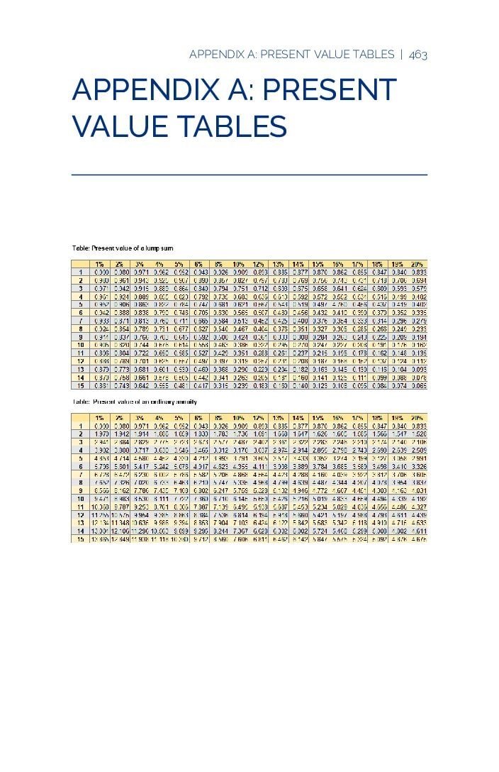
A managerial accounting course builds toward capital budgeting, and capital budgeting decisions – should the company buy the new machine, open the new location, replace the old delivery fleet – all hinge on comparing cash that arrives at different points in time. A dollar received five years from now is worth less than a dollar in hand today, because today’s dollar can be invested and grow. Present value tables exist to make that comparison mechanical rather than requiring a fresh formula calculation every time: instead of computing (1 + i)^-n by hand for every discount rate and time horizon a course might ask about, a student looks up the intersection of a discount rate column and a number-of-periods row and reads off a present value factor, then multiplies that factor by the future cash amount.
Reading a Present Value of $1 Table
The first table used in capital budgeting problems shows the present value of a single lump-sum amount of $1 received at the end of a given number of periods, discounted at a given interest rate. To use it, a student locates the row for the number of periods until the cash is received and the column for the discount rate (the company’s required rate of return, sometimes called the hurdle rate), and the factor at that intersection is multiplied by the actual future cash amount to find its value in today’s dollars. For example, if a table shows a factor of 0.7130 for eight periods at 7 percent, a future receipt of $10,000 in eight years would have a present value of $7,130 today at that discount rate. This single-sum table is the one used for calculating the present value of a machine’s salvage value at the end of its useful life, or any other one-time cash flow that occurs at a specific future date rather than repeating every period.
Reading a Present Value of an Annuity Table
The second table covers an annuity – a series of equal cash flows occurring at the end of each period for a set number of periods, such as the annual net cash inflow a new machine is projected to generate every year of its useful life. Rather than looking up a separate single-sum factor for each year’s cash flow and adding eight numbers together, the annuity table collapses that entire stream into one factor for a given number of periods and discount rate. Multiplying that single factor by one period’s cash flow amount (assuming the amount is the same every period) gives the present value of the whole stream at once. This is the table used in net present value calculations for a piece of equipment expected to generate a steady annual cash inflow, and it is also the table underlying loan amortization and annuity-due problems in a corporate finance course.
How the Glossary Ties the Course Together
The glossary that accompanies a managerial accounting text is best read as a map of the course’s four major units rather than a list to memorize term by term. The first unit, cost behavior, distinguishes a fixed cost – one whose total dollar amount does not change as production volume rises or falls, such as monthly factory rent – from a variable cost, whose total rises and falls with volume even though the per-unit amount stays constant, such as the cost of raw material per unit produced. A mixed cost blends both patterns, which is why the high-low method exists: it isolates the variable and fixed components of a mixed cost by comparing the highest and lowest activity levels observed and treating the difference in total cost as attributable entirely to the change in volume.
Costing Systems and Manufacturing Accounts
The second unit covers how a manufacturer assigns cost to what it produces. Job-order costing tracks direct material, direct labor, and manufacturing overhead separately for each distinct job or batch, recording the totals on a job cost sheet, and it suits businesses that produce customized or low-volume output such as custom furniture or construction projects. Manufacturing overhead itself is every production cost that cannot be traced directly to a specific unit – the factory supervisor’s salary, factory utilities, machine depreciation – and because these costs cannot be traced directly, businesses apply them to jobs using a predetermined overhead rate calculated in advance by dividing estimated total overhead by an estimated allocation base such as direct labor hours or machine hours. As production happens, cost flows through three inventory accounts in sequence: Raw Materials, then Work in Process as material, labor, and applied overhead accumulate on unfinished units, and finally Finished Goods once a job is complete and ready for sale.
Budgeting and Variance Terminology
The third unit shifts from historical costing to forward planning. A master budget is the umbrella term for the full set of interlocking budgets – sales, production, materials purchases, manufacturing overhead, and selling and administrative expenses – that together forecast an organization’s financial position for a future period. A planning budget is prepared before the period begins, using the sales volume management expects to achieve, while a flexible budget takes the same cost formulas but reforecasts them using the volume the organization actually achieved, which makes the flexible budget a fairer benchmark for judging cost control than the original planning budget. Comparing the planning budget to the flexible budget isolates an activity variance, caused purely by selling a different quantity than planned, while comparing the flexible budget to actual results isolates a revenue or spending variance, caused by prices or efficiency that differed from what was budgeted for the volume actually achieved.
Performance Evaluation by Segment
The fourth unit applies these same cost-behavior ideas to evaluating parts of an organization rather than the whole. Segmented income reporting traces revenue and variable costs to the specific division, store, region, or product line that generated them, and fixed costs are split into traceable fixed costs (attributable to one segment, and which would disappear if that segment were eliminated) and common fixed costs (shared across segments, such as the CEO’s salary, which would not disappear even if one segment were dropped). Subtracting a segment’s traceable fixed costs from its own contribution margin yields its segment margin, which is the figure managers use to judge whether a segment is pulling its weight, since it strips out costs the segment’s own operations do not actually control.
Quick Revision Summary
A present value of $1 table converts a single future lump sum into today’s dollars by multiplying the future amount by the table factor found at the intersection of the discount rate and number of periods; a present value of an annuity table does the same for a level, repeating cash flow stream in one step. Fixed costs stay constant in total as volume changes, variable costs stay constant per unit, and mixed costs contain both elements. Job-order costing assigns direct material, direct labor, and applied manufacturing overhead to each job as it moves through Raw Materials, Work in Process, and Finished Goods. A flexible budget restates the planning budget at actual volume, separating activity variances (caused by volume) from revenue and spending variances (caused by price and efficiency). Segment margin equals a segment’s contribution margin minus its own traceable fixed costs, deliberately excluding the common fixed costs the segment does not control.